# What is Dwh.dev?
First Snowflake native data observability solution
## **Dwh.dev - next-gen data lineage for Snowflake**
We provide a unique data lineage solution built especially for Snowflake users.
[**Dwh.dev**](https://dwh.dev) is designed to help data teams easily understand, document, and manage their data flow.
With [**Dwh.dev**](https://dwh.dev), you can search and visualize your data lineage, track data dependencies issues, and better understand your data pipelines.
It's a perfect solution for data engineers, analysts, and scientists who want to boost their productivity and efficiency.
It's easy to start: any type of [**integration**](/integrations) takes about a few minutes!
## **How does it work?**
[**Dwh.dev**](https://dwh.dev) is based on a static analyzer.\
We parse SQL, then compile it into an internal representation and analyze it **automatically**.
We don't use information from Snowflake system tables, which allows us to provide features such as:
* [**Snowflake Marketplace (Native App)**](/integrations/snowflake/snowflake-marketplace-native-app): always up-to-date lineage without external dependencies
* [**Offline mode**](/integrations/snowflake/offline-mode): building data lineage without a direct connection to your database.
* [**In-query lineage**:](/features/data-lineage/in-query-lineage) visualizing the dependency graph within a query.
* [**Equals lineage**](/features/data-lineage/equals-column-lineage): displaying a hidden dependency graph based on conditions in `JOIN` and `WHERE`.
* [**QUERY\_HISTORY analysis and schema change tracking**](/integrations/snowflake/snowflake-marketplace-native-app/query_history-analysis-and-schema-change-tracking)
* [**CTAS cost management**](/integrations/snowflake/snowflake-marketplace-native-app/ctas-cost-management)
* [**CTAS logic change tracking**](/integrations/snowflake/snowflake-marketplace-native-app/ctas-logic-change-tracking)
* [**CTAS logic change alerting**](/integrations/snowflake/snowflake-marketplace-native-app/ctas-logic-change-alerting)
* And much more.
You can access the parsing and compilation results through [**our API**](/integrations/api-offline-mode).
# Features
Although [**Dwh.dev**](https://dwh.dev) is focused on data lineage, the product also has additional features that make life easier for users.\
The main screen is divided into three tabs:
* [**Data Catalog**:](/features/data-catalog) A search system that simplifies working with lineage.
* [**Lineage**](/features/data-lineage): A dependency graph. For small projects (up to 500 connections), it is possible to explore the entire database graph on one screen. For large projects, working with data lineage begins with selecting an object for exploration.
* [**Tasks**](/features/tasks): A dependency graph of TASK objects in the database. You can explore the data lineage generated by each isolated DAG.
# Data catalog
# PIPEs
# Fancy SQL Highlight
The static analyzer provides comprehensive information about all objects and columns at any point in an SQL query, making SQL highlighting more convenient and functional.\
\
In detailed object information and the DDL on the Lineage screen, you can observe SQL highlighting in this manner:
Clickable source objects
Each object has an icon corresponding to its type and is clickable. Clicking on it will take you to the selected object. We distinguish all types of Snowflake objects - TABLE, VIEW, STAGE, STREAM, FUNCTION, etc.
Additionally, we've created a reference guide for core functions. Hovering over such a function in SQL, you'll see a brief description:
Short function's description
Clicking will expand the details and provide a link to the original documentation.
# Data Lineage
# Object-level lineage
# Column-level Lineage
# In-query lineage
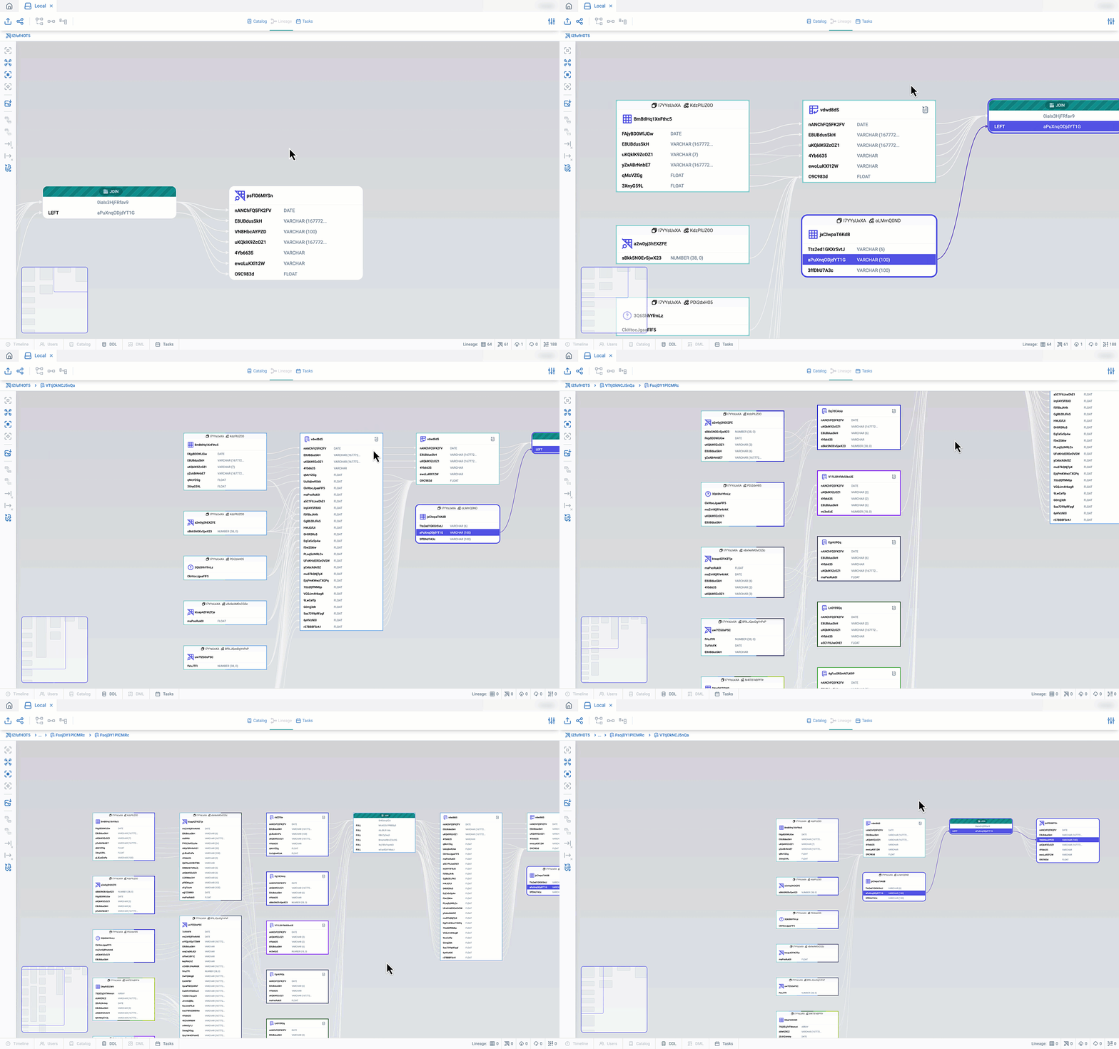
we realized that no matter how accurately we display column-level lineage between objects, on the **"last mile"** (**within CTAS/VIEW queries**), SQL developers are left without help and spend a lot of time exploring complex queries.
We couldn't let this happen, so we developed a new
Now you can go deeper into a selected object's logic and get column-level lineage for the internals of a **SELECT query** with **a** unique feature - **IN-QUERY LINEAGE.**
In-query lineage
In the current "preview" stage, we highlight CTEs, sub-queries, pivots, joins, and unions. We allow collapsing/expanding each sub-query to control the level of detail.
**This functionality is also available for DBT projects.**
# Navigation
[**Youtube**](https://youtu.be/BS0XvzyTnwA)
The commonly accepted navigation standard for Lineage is "expanding" each subsequent level on demand. This involves requesting information about each subsequent level from the backend.
At [**Dwh.dev**](https://dwh.dev/), we took a different approach - dependency information is loaded to the client, allowing us to display the necessary number of levels instantly, rebuilding the graph as needed.
For user's convenience, small graphs (with up to 500 connections) can be displayed entirely. Large graphs are available for exploration only in parts because navigating large graphs is almost impossible.
Initially, through a search, you find the necessary object in the catalog and by clicking the "lineage" button, you enter the "group" of that object.
The main object of the group is highlighted with a dashed border.
The lineage screen supports scaling, scrolling, various types of centering, and a mini-map. You can always return to the main object by clicking the first button in the button group, aligning it in the toolbar, or by the object name in the top right.
To the left of the central object are **Upstream** objects; to the right, **Downstream** objects. **Upstream** objects may have violet circles on the right side of the object. The numbers in these circles indicate the number of objects in **Downstream** that do not belong to the current group. Similarly, there is a green circle on the left of **Downstream** objects, indicating the number of objects from **Upstream** outside this group.
To enter a group of objects on the screen, double-click on it. To go back, press ESC.
By default, 2 levels of lineage are displayed. You can change this value in the settings panel under **Stream Options**:
You can also quickly disable the display of all Upstream/Downstream levels in the toolbar with the **"Toggle stream length to 0"** buttons.
If you want to explore the graph in a "classic" mode, navigating through its levels by "expanding" them, there is a **"Custom Path"** mode for this purpose:
The labels on the edges of the graph show how many levels are hidden in this branch, the number of objects in the first level, and the total number of objects.
You can highlight only the objects that interest you at the moment:
When working with complex graphs, even in **"Custom Path"** mode, it can be challenging to orient oneself. Therefore, you can "straighten" the selected path using the **"Straighten the path"** button in the toolbar:
Both of these modes also work at the column level:
# JOIN and WHERE
Typically, data lineage tools provide information about the immediate movement of data within the database:
```sql
CREATE VIEW v1
AS
SELECT c1
FROM t1
```
Data from the column **t1.c1** flows into **v1.c1**:
However, this data might be insufficient when it comes to refactoring. For instance, when certain columns aren't involved in the data movement but are only involved in **JOIN** or **WHERE** clauses:
```sql
CREATE VIEW v2
AS
SELECT c1
FROM t1
JOIN t2 ON t1.id = t2.parent_id
WHERE
t1.c2 > t2.f2
```
Usually, data lineage tools won't provide information about columns **t1.id, t1.c2, t2.parent\_id, t2.f2**, but at [**Dwh.dev**](https://dwh.dev/), we've made them visible!
# Equals column lineage
We already have great functionality for displaying relationships from [**JOIN and WHERE** ](/features/data-lineage/join-and-where)clauses.
But that's not all.
Remember what we learned in school? If we know that x = y, we can substitute one for the other anywhere. Right? Now, take a look at this query:
```sql
SELECT T1.C1 FROM
T1 JOIN T2 ON T1.C1 = T2.C3
```
We get **T1.C1** as the lineage result, correct?
But **T1.C1 = T2.C3**, which means this query is equivalent to:
```sql
SELECT T2.C3 FROM
T1 JOIN T2 ON T1.C1 = T2.C3
```
See what's happening here? The lineage of the upstream column **T2.C3** is hidden from your view!
Have you ever encountered a tool that reveals this to you? Sure, you'll see that there's a dependency on table T2 at the object level. But no details. Good luck debugging that!
It gets even worse! If x = y and y = z, then x = z. Right?
```sql
SELECT C1 FROM
T1
JOIN T2 ON C1 = C3
JOIN T3 ON C3 = C5;
```
You get the point…
All of this becomes even more complicated when you add mathematical operations, function calls, type conversions, unions…
Can we see additional data lineage generated by the equality conditions in JOIN and WHERE?
Sure! Here's what the full data lineage would look like for the examples above:
Equals lineage #1
Equals lineage #2
# Strong and Weak dependencies
[**Youtube**](https://youtu.be/jQeVVlqxjj8)
In the [**JOIN and WHERE section**](/features/data-lineage/join-and-where), we discussed displaying columns used in JOIN and WHERE clauses. But we wanted to go further :)
Even if columns are data sources, it makes sense to divide them into 2 categories: columns that are direct data sources and columns that only influence them.
For example:
```sql
SELECT
ROUND(a, b)
FROM t
```
Here, column A is a direct data source, while B is not. B influences the result, but A is the primary source.
Another example:
```sql
SELECT
CASE
WHEN A IS NULL
THEN B
ELSE C
END
FROM t
```
Here, the value from A doesn't appear in the result but affects it.
At [**Dwh.dev**](https://dwh.dev/), we divided such dependencies into classes: **STRONG** and **WEAK**. We annotated all core functions to determine which argument belongs to which class. We also analyze CASE WHEN and other cases. You can disable any of these classes in the settings panel:
Weak dependencies
# Default and Virtual Columns
[**Youtube**](https://youtu.be/eLi8CnXP8LA)
**Default and Virtual Columns** also contain information about data lineage. And as usual, nobody pays attention to it :)
```sql
-- default value
CREATE TABLE t1 (
id1 int,
id2 int default (id1 +1)
);
CREATE VIEW v1 AS
SELECT *
FROM t1
;
```
If during data transformations, only the id1 column is inserted into the **T1** table, the lineage information will be lost.
At [**Dwh.dev**](https://dwh.dev/), we display it like this:
With **Virtual columns**, an even more precarious situation arises. It's impossible to insert data into a virtual column, and they will ALWAYS depend on other columns in the table.
```sql
-- virtual column
CREATE TABLE T2 (
A INT,
B INT,
C INT,
D INT AS (CASE WHEN A>0 THEN B ELSE C END)
);
CREATE VIEW v2 AS
SELECT *
FROM t2
;
```
At [**Dwh.dev**](https://dwh.dev/), we display it like this:
# Implicit Types casting
# Circle dependencies
# Argument forwarding
# TASKs
# Integrations
# Snowflake
#### Operation Modes
| [**Snowflake Marketplace (Native App)**](/integrations/snowflake/snowflake-marketplace-native-app) | Runs fully inside your Snowflake account as a native application. All parsing, lineage analysis, and metadata storage happen within your Snowflake environment using Snowflake-managed compute. Supports live schema change tracking and logic change alerting | ✅ Recommended — provides the richest feature set, automatic updates, and integrated billing. |
| -------------------------------------------------------------------------------------------------- | -------------------------------------------------------------------------------------------------------------------------------------------------------------------------------------------------------------------------------------------------------------- | -------------------------------------------------------------------------------------------- |
| [**Offline Mode**](/integrations/snowflake/offline-mode) | Runs as a service in our cloud. Only static SQL files are analyzed; no connection to Snowflake is required. Ideal for isolated environments or CI/CD validation pipelines. | For restricted environments or local development. |
> 💡 We recommend using the Snowflake Marketplace deployment, as it provides the most complete functionality — including live lineage synchronization, compute-pool execution, governance integration, and seamless billing via your Snowflake account balance.
# Snowflake Marketplace (Native App)
Always up-to-date lineage without external dependencies
#### Overview
DWH.dev is available directly in the [Snowflake Marketplace](https://app.snowflake.com/marketplace/listing/GZTSZ1Y553M/dwh-dev-inc-dwh-dev-lineage) as a native application.
This allows you to deploy and run DWH.dev ***inside your own Snowflake account***, without sharing data externally or managing any external infrastructure.
The Marketplace version of DWH.dev performs static SQL analysis and metadata lineage computation directly in your Snowflake environment - leveraging the same security, governance, and role-based access controls you already use.
***
#### Benefits of Marketplace Deployment
* **100% Snowflake-native** - no data leaves your account
* **Instant setup** - no servers or containers to manage
* **Secure** - fully isolated within your Snowflake account without external dependencies
* **Automatic updates** - always the latest version
* **Continuously up-to-date lineage** - DWH.dev refreshes lineage automatically based on schema change tracking
* **Integrated billing** - usage is billed through your existing Snowflake account balance (no separate contracts or credit cards)
#### Requirements & Resources
| **Snowflake Account** | Any account tier starting from **Standard** | No dependency on [ACCESS\_HISTORY view](https://docs.snowflake.com/en/sql-reference/account-usage/access_history) — DWH.dev performs *static* SQL analysis |
| --------------------- | ------------------------------------------------------------------------------ | ------------------------------------------------------------------------------------------------------------------------------------------------------------------ |
| **Compute Pool** | DWH.dev runs entirely inside a dedicated compute pool of size **CPU\_X64\_S** | Adds credit utilization of \~0.11 credits/hour, as per [Snowflake Credit Consumption Table (1d)](https://www.snowflake.com/legal-files/CreditConsumptionTable.pdf) |
| **Warehouse** | M size | Used for query-history export |
| **Permissions** | Metadata read access on target databases and Read access to **QUERY\_HISTORY** | No SELECT access to data contents required. |
| **Network Access** | None required | fully in-account execution |
#### Features
* [QUERY\_HISTORY analysis and schema change tracking](/integrations/snowflake/snowflake-marketplace-native-app/query_history-analysis-and-schema-change-tracking)
* [CTAS cost management](/integrations/snowflake/snowflake-marketplace-native-app/ctas-cost-management)
* [CTAS logic change tracking](/integrations/snowflake/snowflake-marketplace-native-app/ctas-logic-change-tracking)
* [CTAS logic change alerting](/integrations/snowflake/snowflake-marketplace-native-app/ctas-logic-change-alerting)
# QUERY\_HISTORY analysis and schema change tracking
# CTAS cost management
{% embed url="" %}
DWH.dev automatically identifies all `CREATE TABLE AS SELECT` (CTAS) operations and links them to their corresponding compute cost using data from Snowflake’s `QUERY_HISTORY`.\
Each CTAS execution is associated with its target object, warehouse, and runtime metadata — allowing DWH.dev to estimate and attribute the credit consumption of transformation pipelines.
Costs are calculated based on the warehouse type used during execution (e.g., `XSMALL`, `MEDIUM`) and the runtime duration recorded in `QUERY_HISTORY`.\
In native Marketplace deployments, this data is enriched with compute-pool utilization metrics, providing a unified view of both **warehouse** and **pool-level** resource usage.
#### Used for
* Identifying the most expensive CTAS transformations across your pipelines.
* Tracking warehouse utilization and compute-pool credit consumption.
* Optimizing task schedules and warehouse configurations to reduce recurring costs.
* Highlighting redundant or rarely used CTAS operations.
# CTAS logic change tracking
{% embed url="" %}
DWH.dev tracks logical changes in `CREATE TABLE AS SELECT` (CTAS) operations based on data from Snowflake’s `QUERY_HISTORY`.\
For every CTAS statement, the corresponding target object is identified, and its `query_hash` — the unique identifier of the compiled query generated by Snowflake — is extracted.
If the current `query_hash` differs from the previously stored one, DWH.dev flags this as a **CTAS logic change** and automatically recalculates all dependent lineage relationships.\
This means that even when the table name remains unchanged, any modification in the SQL logic (such as added columns, altered joins, filters, or expressions) is immediately reflected in the lineage graph.
#### Used for
* Tracking the evolution of transformation logic over time.
* Auditing business-logic changes without manually comparing SQL code.
* Automatically updating lineage whenever CTAS logic changes.
* Preventing silent downstream inconsistencies caused by logic drift.
# CTAS logic change alerting
{% embed url="" %}
# Offline mode
[**Dwh.dev**](https://dwh.dev/) allows you to work without a direct connection to your **Snowflake** instance.
Typically, data lineage tools require information from the **INFORMATION\_SCHEMA**, which is only accessible through a direct connection to your account.
However, we independently compile the schema into an intermediate representation, requiring only the file with DDL statements. This opens up several possibilities:
* You can explore the lineage of only the part of the database that is available to you, without going through all the security procedures adopted in your company when creating a user for a direct connection.
* You can explore the lineage of a database to which you do not have access, but there is a schema description.
* You can upload schema descriptions for multiple databases at once.
To use offline mode, execute the following SQL query in your account:
```sql
SELECT GET_DDL('database', '', TRUE);
```
and upload the result to [**Dwh.dev**](https://dwh.dev/).
However, this approach has some downsides:
1. Not all objects of interest can be obtained with this command, and some objects are returned incorrectly. For example, if a **STREAM** is created for an object from another schema, **GET\_DDL** will return an error description. We recommend enriching the results of the **GET\_DDL** function with additional functions from our collection:
2. The commands in the results of the **GET\_DDL** function are sorted in alphabetical order of object names. For example, if **VIEW v1** depends on **VIEW v2**, you won't be able to run the resulting set of statements without errors. **The good news** is that we can topologically sort DDL statements before compilation. When uploading the file, specify that you are uploading the result of the **GET\_DDL** function, and we will take care of the rest :)
You can also upload files with sets of DML and DDL statements describing your **PIPELINES**. You can retrieve them from **QUERY\_HISTORY** if you do not store them separately.
If you have sets of SELECT statements describing **BI REPORTS**, you can also upload them yourself.
We will also include information about relationships and objects from these files in the overall lineage and catalog.
# DBT
# API (offline mode)
# Snowflake SQL Syntax and Behavior
[**Dwh.dev**](https://dwh.dev/) team has been dealing with SQL static analysis for a long time, and we know very well that all databases behave differently: unique SQL syntax, object types, and relationships, and peculiar behavior of seemingly obvious things.
Snowflake documentation often describes not all the nuances of a database's behavior, or yet sometimes it simply doesn't match the actual state of affairs.
In this section, we provide examples of special behavior and SQL syntax and show how [**Dwh.dev**](https://dwh.dev) handles these complexities.
# Identifiers
## Basic Syntax ([Youtube](https://youtu.be/RIfgdpIOA3Q))
**Snowflake** provides an extensive toolkit for working with object and column identifiers. Let's start with the basics: identifiers with and without quotes ([documentation](https://docs.snowflake.com/en/sql-reference/identifiers-syntax))
Even at this stage, we won't achieve full compatibility with the syntax of other databases. However, two nuances deserve special attention:
* Identifiers without quotes are converted to uppercase.
* Identifiers within backticks behave similarly.
```sql
CREATE TABLE `Myidentifier` (
f5 INT
);
CREATE TABLE "quote""andunquote""" (
f6 INT
);
```
We collected all the varieties of the basic syntax [in 1.identifiers.1.sql](https://github.com/dwh-dev/data-lineage-challenge/blob/main/snowflake/1.identifiers/sql/1.identifiers.1.sql)
Here is the [**Dwh.dev**](https://dwh.dev/) result:
## Special syntax ([Youtube](https://youtu.be/hGf2VtBxzHU))
In addition to the basic syntax, **Snowflake** has special functionality:
* [Literals and Variables as Identifiers](https://docs.snowflake.com/en/sql-reference/identifier-literal). A special **IDENTIFIER()** function to get a reference to an object or column from a session variable or string.
* [Table Literals](https://docs.snowflake.com/en/sql-reference/literals-table) Special function **TABLE()** to get a reference to an object from a session variable or string.
* [Double-Dot Notation](https://docs.snowflake.com/en/sql-reference/name-resolution#resolution-when-schema-omitted-double-dot-notation) A special syntax that allows the **PUBLIC** scheme to be omitted when addressing an object.
```sql
CREATE VIEW V1 AS
SELECT *
FROM
identifier($table_var1)
;
-- Column Identifier
CREATE VIEW V4 AS
SELECT identifier('DEMO_DB.SCH1.T1.V1'):json_prop as prop
FROM
DEMO_DB.SCH1.T1
;
-- Double-Dot Notation
CREATE VIEW V8 AS
SELECT *
FROM
DEMO_DB..T3
;
```
This syntax is often found in the description of transformations because it helps to use the same source code with different object names.
We have collected all kinds of special syntax [in 1.identifiers.2.sql](https://github.com/dwh-dev/data-lineage-challenge/blob/main/snowflake/1.identifiers/sql/1.identifiers.2.sql).
Here is the [**Dwh.dev**](https://dwh.dev/) result:
# Reusing column aliases
In any database, you can use aliases for both columns and expressions within queries:
```sql
SELECT
id AS user_id,
name AS user_name,
age AS user_age,
age * 2 AS user_age_doubled
FROM users;
```
But what can we do with these aliases? Database vendors allow different things. For example, in MySQL and PostgreSQL, aliases can only be used in **GROUP BY** and **ORDER BY**. In Clickhouse and **Snowflake**, however, aliases can be used everywhere. But, as usual, there are nuances :)
Let's create syntactically identical VIEWs:
```sql
CREATE TABLE abc AS SELECT 1 AS a, 100 AS b, 1000 AS c;
CREATE VIEW v13 AS
SELECT
a+1 AS b,
b+1 AS c
FROM abc;
CREATE VIEW v14 AS
SELECT
a+1 AS d,
d+1 AS e
FROM abc;
```
At first glance, the lineage for these views should be the same. But let's see what happened:
Why in **V13** the column **C** not reuse the alias **B**? Because in **Snowflake** when using an alias equivalent to the original column name from the source, the original column takes precedence!
By the way, in Clickhouse, it works differently...
What was meant by saying that aliases work everywhere?
Aliases can be reused in JOIN and WHERE clauses:
```sql
CREATE TABLE t12 AS SELECT 1 AS a, 100 AS b;
CREATE TABLE t13 AS SELECT 1 AS c, 100 AS d;
CREATE VIEW v15 AS
SELECT
a + b AS e,
c + d AS f
FROM
t12
JOIN t13 ON e = f;
```
or even like this:
```sql
CREATE VIEW v16 AS
SELECT
a1 + b1 AS e,
c1 + d1 AS f,
ROUND(e, f) AS g,
ROUND(f, e) AS h
FROM
t12 AS t121(a1, b1)
JOIN t13 AS t131(c1, d1) ON e = f
WHERE
g = h;
```
Since in [**Dwh.dev**](https://dwh.dev/) we display not only the data flows but also the [**columns used in JOIN and WHERE**](/features/data-lineage/join-and-where), you will also see the original column sources in the corresponding section.
# SELECT \* ILIKE EXCLUDE REPLACE RENAME
Database vendors are competing to see who can come up with the most features for **SELECT \***. **Snowflake** is not lagging and supports as many as 4 modifiers for **SELECT \***:\
**ILIKE EXCLUDE REPLACE RENAME**
We all know that **SELECT \*** is bad. Now it's 4 times worse :)\
Ok, 3. You can't use them all together (either **ILIKE** or **EXCLUDE**).
But the most disgusting modifier is **REPLACE**. It allows you to replace one column with any expression. Good luck debugging, dudes :)
What happens to lineage when using these modifiers? A few examples are collected here: [in 4.select-ilike-exclude-replace-rename.1.sql](https://github.com/dwh-dev/data-lineage-challenge/blob/main/snowflake/4.select-ilike-exclude-replace-rename/sql/4.select-ilike-exclude-replace-rename.1.sql)
Take a look at one of them:
```sql
CREATE TABLE t19(
id INT,
c1 BOOLEAN,
c2 BOOLEAN,
c3 BOOLEAN,
c4 BOOLEAN,
c12c BOOLEAN
);
CREATE TABLE t20(
c5 BOOLEAN,
c6 BOOLEAN
);
CREATE VIEW v20 AS
SELECT
*
ILIKE 'c%'
REPLACE (a.c1 OR b.$2 AS c1)
RENAME c1 AS c0
FROM t19 a, t20 b
;
```
At [**Dwh.dev**](https://dwh.dev/), we display it like this:
# Scalar functions name resolution special behavior
This topic is about the behavior of name resolution in Snowflake inside **CREATE VIEW**.
When you execute queries, Snowflake looks for the objects specified in the query in the schemas specified in **SEARCH\_PATH**. You can view them like this:
```sql
SELECT current_schemas();
```
But it seems like a good idea to make the creation of VIEWs independent of **SEARCH\_PATH**. Otherwise, we will get different results when we work with VIEWs at different **SEARCH\_PATH**.
The documentation says the following:
> The **SEARCH\_PATH** is not used inside views or UDFs. All unqualifed objects in a view or UDF definition will be resolved in the view’s or UDF’s schema only.
That's great! And it works!
```sql
CREATE OR REPLACE DATABASE db1;
CREATE SCHEMA sh1;
CREATE TABLE public.t1(c1 int);
CREATE VIEW sh1.v1 AS
SELECT * FROM t1;
```
will return
```sql
SQL compilation error:
Object 'DB1.SH1.T1' does not exist or not authorized.
```
And not only for tables. For any objects, except … **scalar functions**!
```sql
CREATE OR REPLACE DATABASE db1;
CREATE SCHEMA sh1;
CREATE TABLE sh1.t1(c1 int);
INSERT INTO sh1.t1(c1) VALUES (1);
CREATE FUNCTION public.test()
RETURNS NUMBER
LANGUAGE SQL
AS '1';
CREATE VIEW sh1.v1 AS
SELECT *, test() c2 FROM t1;
select * from sh1.v1;
```
will return
```sql
C1 C2
1 1
```
Strange behavior, don't you agree?
In PostgreSQL, for example, it works like this: when creating a VIEW, all objects without schema specification are searched in the public schema. If you want a different schema, specify it by hand.
But maybe I'm being picky? Let's add one more thing…
```sql
CREATE FUNCTION sh1.test()
RETURNS NUMBER
LANGUAGE SQL
AS '2';
select * from sh1.v1;
```
will return
```sql
C1 C2
1 2
```
Oops… i.e. if there is a scalar function in the scheme where **VIEW** is created, it will be used. If not, the function from **PUBLIC** will be used.
**I.e. if you didn't specify a schema for a scalar function from the PUBLIC schema while creating a VIEW, in a schema other than PUBLIC, then to corrupt the data in your database it is enough to create a function with the same name in the corresponding schema…**
At [**Dwh.dev**](https://dwh.dev/), we don't display downstream lineage for scalar functions right now, but if you click on that function in the source code ([**which we display in a very cool way**](/features/data-catalog/fancy-sql-highlight)), you will jump to the exact function used in that context.
# Functions overloading
Snowflake support [procedures and functions overloading](https://docs.snowflake.com/en/developer-guide/udf-stored-procedure-naming-conventions#overloading-procedures-and-functions). You can create multiple UDFs with the same name but with different types of arguments..
Let's create:
```sql
CREATE TABLE A(ID INT);
CREATE TABLE B(S STRING);
CREATE OR REPLACE FUNCTION fn_overload ( _id number )
RETURNS TABLE (id int)
AS 'select id from a where id > _id'
;
CREATE OR REPLACE FUNCTION fn_overload ( _s string )
RETURNS TABLE (s string)
AS 'select s from b where s != _s'
;
```
The first one has **Table A as a source**, and the second one **Table B**.
Now let's create VIEWs depending on these functions:
```sql
CREATE VIEW V1 AS
SELECT * FROM TABLE(fn_overload(1));
CREATE VIEW V2 AS
SELECT * FROM TABLE(fn_overload('1'));
```
Here is the [**Dwh.dev**](https://dwh.dev/) result:
# CTE as an expression alias
We all like to use **CTEs (Common Table Expression)**. It makes our code cleaner and sometimes helps to speed up queries.
But somehow, Snowflake documentation hides from us one beautiful behavior of CTE that will make your life even more convenient.
What does the [documentation say](https://docs.snowflake.com/en/user-guide/queries-cte)?
> A CTE (common table expression) is a named subquery defined in a WITH clause. You can think of the CTE as a temporary view for use in the statement that defines the CTE
In other words:
* we can only use SELECT in the CTE
* the result of the CTE is a view-like object
Surely many of you have used the CTE to define some constants that are used further in the query. For example:
```sql
WITH
var_cte AS (
SELECT 'Snowflake' AS vendor
)
SELECT *
FROM t
WHERE
vendor = (SELECT vendor FROM var_cte)
```
Tolerable, but not perfect. Especially scalar sub-queries. Scalar sub-queries are bad practice. Avoid using them!
Can this be done more elegantly? Yes! Look at this:
```sql
WITH
var_cte AS ('Snowflake')
SELECT *
FROM t
WHERE
vendor = var_cte;
```
Wow! The code became easier to read, and we got rid of scalar sub-queries at the same time!
What if we want to use several values at once? We can make an object:
```sql
WITH
var_cte AS ({'vendor': 'Snowflake'})
SELECT * FROM t WHERE
vendor = var_cte:vendor;
```
Or here's the IN analog:
```sql
WITH
var_cte AS (['Snowflake', 'Bigquery'])
SELECT * FROM t WHERE
ARRAY_CONTAINS(vendor::VARIANT, var_cte)
```
Although it's not so beautiful anymore…
It turns out that CTE can be not only a view-like object but also a scalar value!
Very cool, but even this is not a final:
```sql
CREATE TABLE t AS SELECT 1 AS a, 2 AS b;
WITH
var_cte AS (a+b)
SELECT
var_cte
FROM t;
```
As a result, we will get a table with a var\_cte column and a value of 3.
**I.e. CTE is not only a view-like object, and not only a scalar value but also an alias to any expression!**
Here's another example:
```sql
WITH
var_cte AS (SUM(a))
SELECT
var_cte
FROM t;
```
Yes, you can use any function calls there, including aggregate function calls.
And even that works too:
```sql
WITH
var_cte1 AS (a),
var_cte2 AS (var_cte1+b)
SELECT
var_cte2
FROM t;
```
And like a function's argument:
```sql
WITH
var_cte AS (a + b)
SELECT
ROUND(var_cte/2, 0)
FROM t;
```
Are there any downsides? Unfortunately, yes… First of all, CTE macros refuse to work when you use them in UNION and inline FROM queries:
```sql
-- doesn't work!
WITH
var_cte AS (a+b)
SELECT var_cte FROM t1
UNION
SELECT var_cte FROM t2
;
-- and here
WITH
var_cte AS (a)
SELECT * FROM (
SELECT var_cte FROM t
);
```
Maybe Snowflake engineers will finish this functionality and CTE macros will become possible to use everywhere. Let's hope they know about it themselves :)
And second, none of the data lineage tools will tell you that.
But the good news is that in [dwh.dev](https://dwh.dev/) we take CTE macros into account at compile time and display all relevant connections in lineage!
PS: I found out about it quite by accident from the last example in the [documentation of the ENCRYPT\_RAW function](https://docs.snowflake.com/en/sql-reference/functions/encrypt_raw#examples)
# ASOF Join
Perhaps not everyone knows, but Snowflake now has a new type of connection with an additional condition - [**ASOF JOIN**](https://docs.snowflake.com/en/sql-reference/constructs/asof-join).
> An ASOF JOIN operation combines rows from two tables based on timestamp values that follow each other, precede each other, or match exactly. For each row in the first (or left) table, the join finds a single row in the second (or right) table that has the closest timestamp value. The qualifying row on the right side is the closest match, which could be equal in time, earlier in time, or later in time, depending on the specified comparison operator.
```sql
SELECT l.c1 as a, l.c4 as b, r.c4 as c
FROM left_table l ASOF JOIN right_table r
MATCH_CONDITION(l.c3>=r.c3)
ON(l.c1=r.c1 and l.c2=r.c2)
ORDER BY l.c1, l.c2
```
The **MATCH\_CONDITION** is now displayed next to the **ON** condition in the [**in-query lineage**](/features/data-lineage/in-query-lineage). All columnar relationships are highlighted on click:
# UDF named arguments
# Objects auto renaming
# Columns auto renaming